Background

In this post I describe neural networks as well as provide mathematical derivations of the back-propagation algorithm (commonly used to train neural networks) from ground up. I also discuss and provide a practical and modular C++ implementation of of neural networks.

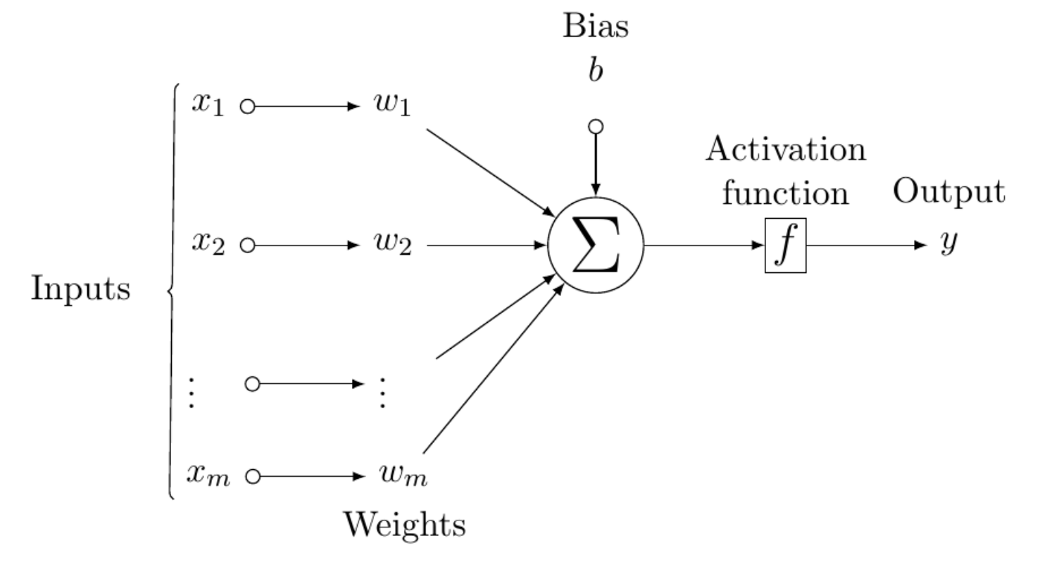
Figure 1: The perceptron. A single neural processing unit. The inputs are multiplied with corresponding weights and linearly combined. The result is then fed to the activation functin to produce the output.

McCulloch and Pitts introduced the idea of biologically inspired computing machines known as neural networks. Building on the McCulloch and Pitts idea, Rosenblatt proposed the perceptron as the first model of learning with examples (supervised learning), called the McCulloch-Pitts model of a neuron. The neural model consists of a linear combiner and a hard limiter as shown in Figure 1.

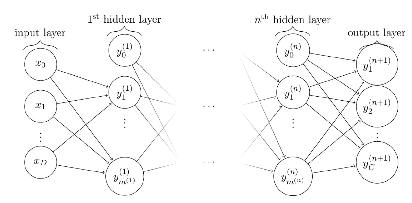
A single layer neural network as described above, Figure 1, is of limited practical use; it can only do classification for linearly separable patterns. In the real world, neural network designs consider neural networks with more than one layer—multilayer perceptrons, see Figure 2. Multilayer perceptrons are characterized by the following features:

• One or more hidden layers (they are hidden from both input and output layers)
• Differentiable nonlinear activation function for each neuron
• High a degree of connectivity The above mentioned characteristics of multilayer perceptrons make it to understand the behavior of neural networks: High connectivity and nonlinearity, for example, are difficult to analyze theoretically, and it is challenging to acquire a good intuition of the learning process of hidden layers since they are difficult to visualize.

In this post, I am going to focus only on feed-forward neural networks.

Figure 2: A feed forward neural network activation flows from one layer to immediate “down-stream” layer. A demonstration of a multilayer perceptron with D inputs and C output “neurons”.

A neural network architecture is “feed-forward” when nodes within a particular layer are connected only to nodes in the immediately “down-stream” layer. In this way, nodes in the input layer only activate nodes in the subsequent hidden layer. The subsequent hidden layer, in turn, will only activate nodes in the next hidden layer. This remains true until the nodes of the most down-stream hidden layer. The most down-stream hidden layer then feeds the output layer; see illustration in Figure 2. While every node is connected to every node in, as shown in Figure 2, layers are not generally fully connected. Nodes from some layer, say i that innervate the $j^{th}$ node in the subsequent layer j are in general a subset of the $\textbf{I}$ nodes that constitute the $i^{th}$ layer. We denote this subset by $\textbf{I}_k$. So the weighted sum of the inputs is described as:

where $\textbf{I}_j$ is the set of nodes from the $i^{th}$ layer which feeds node j.

The Back-propagation Algorithm: On-line Training of Multilayer Perceptrons

Recall, as per discussion in the previous section, that feed-forward neural networks on which the backpropagation learning algorithm is deployed consist of layers classified as input, hidden, and output. In this configuration, there is only one input layer and one output layer. The number of hidden layers is only limited by available computing resources.

The back-propagation algorithm is the most popular method by which neural networks are trained. Training with the back-propagation proceeds in two phases:

1. Forward phase—in this phase the synaptic weights of the network are fixed and the input signal is propagated through the network on al yer by layer basis until it reaches the output layer.
2. Backward phase—in this phase, first an error signal is produced by comparing the output of the network and a known desired response. The resulting error signal is then propagated through the network, layer by layer in the backward direction. In this phase adjustments to weights are made to synaptic weights of the neural network.

Fundamentally, a supervised learning algorithm attempts to minimize the error between the actual output values (activations at the output layer for neural networks) and the desired values. The algorithm achieves this objective by changing the values of the weights in the network. Because the back–propagation is an iterative algorithm, weights change incrementally. The change in weight is proportional to its influence on the error: the bigger the influence of weight $w_i$, the larger the reduction of error induced by changing the weight. In other words, the bigger the change our learning algorithm should make in that weight. Note that this influence is not the same everywhere (and in somes cases some weights are fixed by design and never change throughout the training process), and changing any particular weight generally makes all the other weights more or less influential on the error. The process of adjusting weights is repeated until the error falls below some desired threshold, at which point the algorthim is considered to have learned the function of interest and the procedure terminates. For this reason, the back–propagation is also known as a steepest descent algorithm.

Derivation

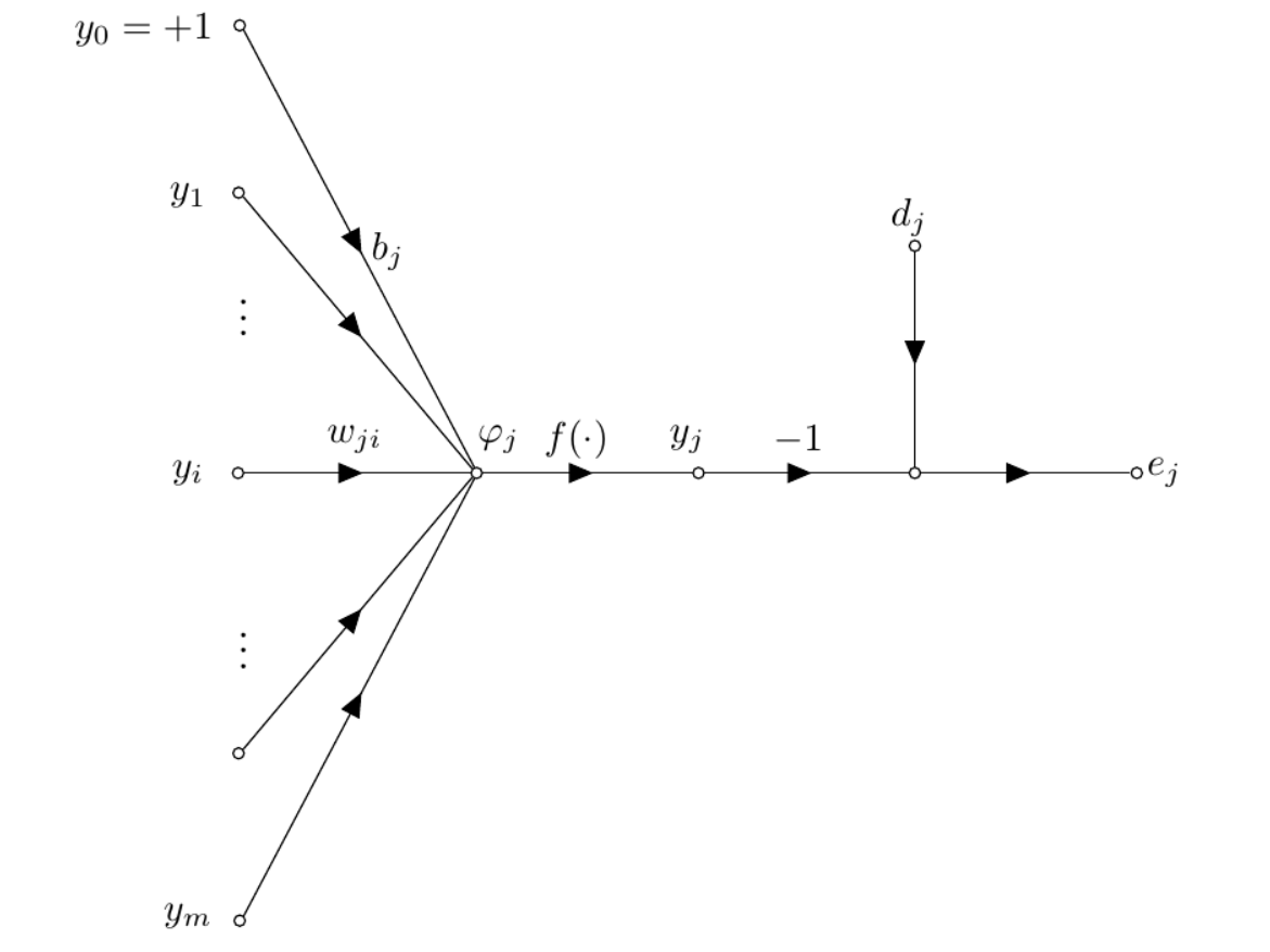
Figure 3: Neural network graph. Demonstration of backpropagation training with a single neural processing unit given a training dataset and computation of the error between desired and neuron output.

Figure 3 illustrates a neuron, j, being fed by a set of input neurons in the previous layer ($i^{th}$). The induced local field $φ_j$ associated with neuron j is described as,

where m is the number of neuronal inputs applied to neuron j. So $y_j$ is the output of neuron j at some iteration n, is defined as;

where f (·) is the activation function. To describe the back-propagation algorithm, let’s suppose that D = {x, d} is a set of example data. As shown in Equation \ref{eq:output}, $y_j$ is the output of neuron j in the output layer due to some input or simulus x. The error between desired value and neuron output is expressed as;

Loss Function

We need to define a meaure of error for our back–propagation algorithm; we consider the error energy at each output node. It ensures that positive and negative errors do not canel each other out. We modify Equation \ref{eq:err} by square the differences before summing them. In addition, we scale the sum of errors by 1/2 for convenience:

Note that \ref{eq:err_sq} assumes that the $j^{th}$ layer is the output layer.

The back-propagation updates synaptic weight $w_{ji}$ with weight correction $\Delta w_{ji}$, which is proportional to the following partial derivative: $\frac{\partial E}{\partial w_{ji}}$.

By the chain rule, we expand the above partial derivative as follows:

where $\varphi_j$ is the weigted sum of inputs into the $j(^{th})$ node. The partial derivative $\partial E / \partial w_{ji}$ represents a sensitivity factor for determining the direction of the search in the weight space for synaptic weight $w_{ji}$.

The above derivations suggest that the error signal plays a key role in computing the weight correction at the output neuron j. Depending on where neuron j is located within the network determines how we deal with the correction, $\Delta w_{ji}$. If neuron j is an output node, like other output nodes, it is supplied with the corresponding desired output and this simplifies calculation of the error signal, and hence the local gradient. However if neuron j is a hidden node (part of a hidden layer), it is not trivial to determine the error. For instance, there is no specified desired output and we cannot compute the error directly. Instead, the error is computed recursively and working backwards in terms of the errors of all the neurons to which the hidden neuron is directly connected.

Differentiating both sides of Equation \ref{eq:err_sq} with respect to $e_j$ we get

Differentiating Equation \ref{eq:err} with respect to $y_j$, we get

Differentiating Equation \ref{eq:output} with respect to $\varphi_j$ yields

Differentiating the induced local field, Equation \ref{eq:local_field}, with respect to $w_{ji}$ gives,

Subsitituting Equations \ref{eq:err_diff}-\ref{eq:local_field_diff} in \ref{eq:chain_rule} gives

Arrange things here The change in a weight connecting a node in the previous layer to a node in layer j is defined by,

Note that $\alpha$ is a free parameter (learning rate) that we set at the beginning of training. With $\alpha$, we can set the step size that is appropriate for the problem at hand. The adjustment of $\alpha$ between values of 0 and 1–is usually ad-hoc. The negative sign in the formular suggestes that the weights change in the direction of decreasing error. \(\begin{equation} \frac{\partial \varphi_j}{\partial w_{ji}} = y_i. \label{eq:partial_local_field} \end{equation}\)

Note that the correction applied to $w_{ji}$, see \ref{eq:weight_change} attempts to minimize the error E via gradient descent in the weight space. Using Equation \ref{eq:partial_err_weight2} in Equation \ref{eq:weight_change} gives the following;

where the local gradient $\delta_j$ is given by

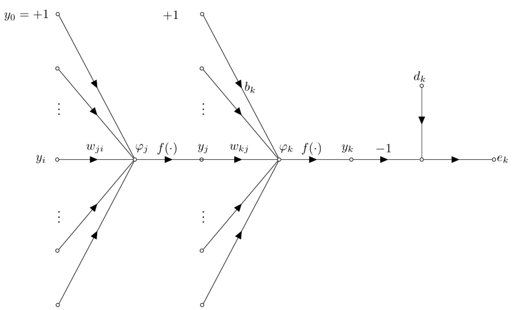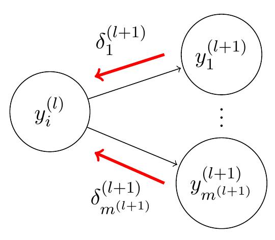
Figure 4: Back-propagation on a neuron located in a hidden layer.

Case A: Neuron is an Output Node

Suppose that neuron j is an output node. Then it is suplied with a corresponding desired or target value. In this case, we may rely on Equation \ref{eq:err} to compute the error $e_j$ associated with the neuron. This makes computing the local gradient $\delta_j$ trivial.

Case B: Neuron is a Hidden Node

When neuron j is part of a hidden layer of the neural network, no desired response is specified for this neuron. Instead, the error signal has to be determined recursively and working backwards in terms of the error of all neurons to whic the hidden neurin is directly connected. Consider scenario as shown in Figure 4 First, we redefine the local gradient based on Equation \ref{eq:local_grad_expand} as follows:

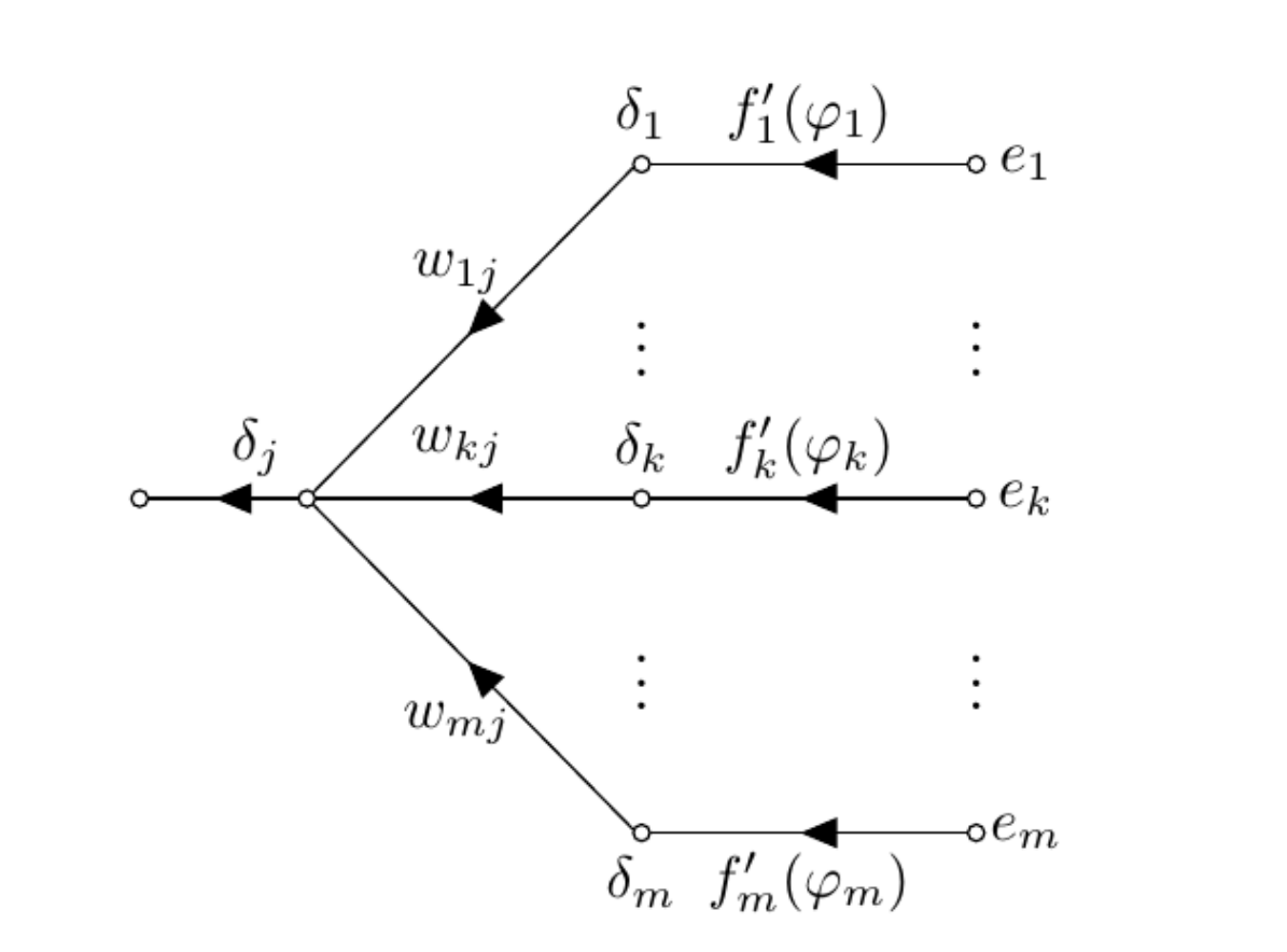Figure 5: Training the perceptron. Demonstration of backpropagation training with a single neural processing unit given a training dataset.

Figure 5: Training the perceptron. Demonstration of backpropagation training with a single neural processing unit given a training dataset.

C++ Implementation of Our Neural Network

Now that etct etc…